Introduction to Statistics

What is Statistics?

• Statistics is the science of collecting, analyzing, interpreting, and drawing conclusions from data. It equips you with tools to understand trends, patterns, and relationships hidden within numbers.

• Statistics is about making sense of data, drawing meaningful conclusions, and uncovering hidden patterns. It goes beyond just summarizing data to understanding its relationship to the real world. Some fundamental statistical concepts are population, sample, variable, and parameter.

Example: How statistics helped predict an election outcome, optimize marketing campaigns, or improve medical treatments

Why Statistics?

In today’s data-driven world, analyzing information effectively is crucial. Statistics paired with Python empowers you to:

• Make informed decisions: Use data to support arguments, validate ideas, and optimize strategies.

• Uncover hidden insights: Explore beyond the surface to reveal fascinating patterns and trends.

• Solve real-world problems, Statistics has a siginificat impact on many fields: ▪ Finance: Predicting market trends, managing risk. ▪ Healthcare: Developing effective treatments, personalizing medicine. ▪ Social Sciences: Understanding social phenomena, informing policy decisions. ▪ Marketing: Targeting customers effectively, measuring campaign performance. ▪ Technology: Building intelligent systems, improving user experience.

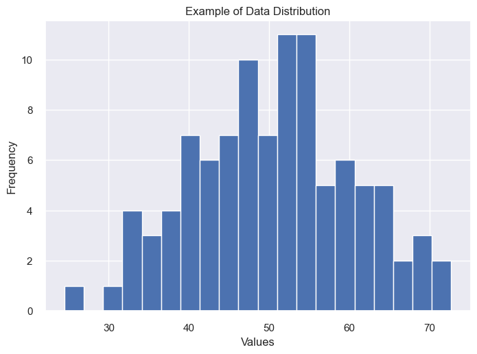
# Example: Generating and visualizing random data
np.random.seed(0)
data = np.random.normal(loc=50, scale=10, size=100)
plt.hist(data, bins=20)
plt.title('Example of Data Distribution')
plt.xlabel('Values')
plt.ylabel('Frequency')
plt.show()

Figure (1): Example of Data Distribution.

Type of Statistics

• Descriptive statistics: Summarizes data using measures like mean, median, mode, standard deviation, frequency tables, and histograms.

  • Helps answer questions like “What is the average age of customers?” or “How many website visitors come from each country”.

• Inferential statistics: Allows us to draw conclusions about populations based on samples. Uses methods like hypothesis testing, confidence intervals, and correlation analysis.

  • Helps answer questions like “Is there a significant difference in product preferences between age groups?” or “Is there a correlation between study hours and exam scores?”

• Example: Predicting exam scores using descriptive statistics (average class score) vs. inferential statistics (sample of students to predict population performance).

Each measure represents data differently and provides different insights:

• Mean (average): Sum of all values divided by the number of values, Represents the “center” of the data. sensitive to outliers.

• Mode: Most frequent value.

• Median: Middle value when data is ordered. Less sensitive to outliers than the mean.

• Variance: Measures how spread out data is from the mean. A higher variance indicates more spread. Calculated as the average of the squared differences between each data point and the mean.

• Standard Deviation: The square root of the variance. Represents the average deviation of data points from the mean. square root makes it more interpretable.

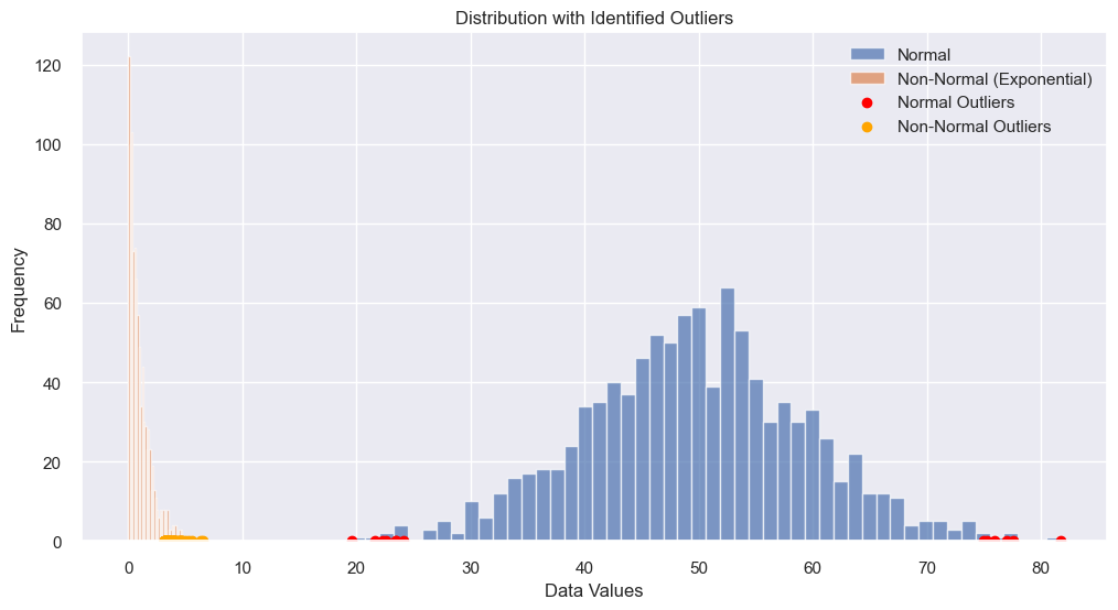
• Outliers: Data points significantly different from the majority. Can distort analysis if not treated carefully.

# Generate example data
data = np.random.normal(loc=50, scale=10, size=100)

Let’s break down the parameters:

• loc=50: This is the mean of the normal distribution. In other words, the center of the distribution is located at 50.

• scale=10: This is the standard deviation of the normal distribution. It measures the spread or “width” of the distribution. A larger standard deviation will result in a wider spread of values around the mean.

• size=100: This is the number of random numbers that you want to generate. Here, it’s set to 100, so the np.random.normal() function will return an array of 100 numbers.

Descriptive Statistics

# Descriptive Statistics
print("Descriptive Statistics:")
print("Mean:", np.mean(data))
print("Median:", np.median(data))
mode_result = stats.mode(data)
if isinstance(mode_result.mode, np.ndarray):
    # If there are multiple modes, print all of them
    print("Mode:", ", ".join(map(str, mode_result.mode)))
else:
    # If there's a single mode, print it
    print("Mode:", mode_result.mode)
print("Standard Deviation:", np.std(data))
print("Variance:", np.var(data))
print("Range:", np.max(data) - np.min(data))
print("Interquartile Range (IQR):", stats.iqr(data))

# Output:
"""
Descriptive Statistics:
Mean: 50.82012970747838
Median: 50.24654858649704
Mode: 27.765968477755735
Standard Deviation: 10.346669974384227
Variance: 107.05357955882408
Range: 46.065479270883685
Interquartile Range (IQR): 15.929097046733524
"""

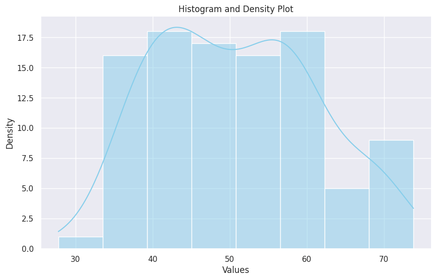
# Histogram and Density Plot (Descriptive Statistics)
plt.figure(figsize=(10, 6))
sns.histplot(data, kde=True, color='skyblue')
plt.title('Histogram and Density Plot')
plt.xlabel('Values')
plt.ylabel('Density')
plt.show()

Figure (2): Histogram and Density Plot.

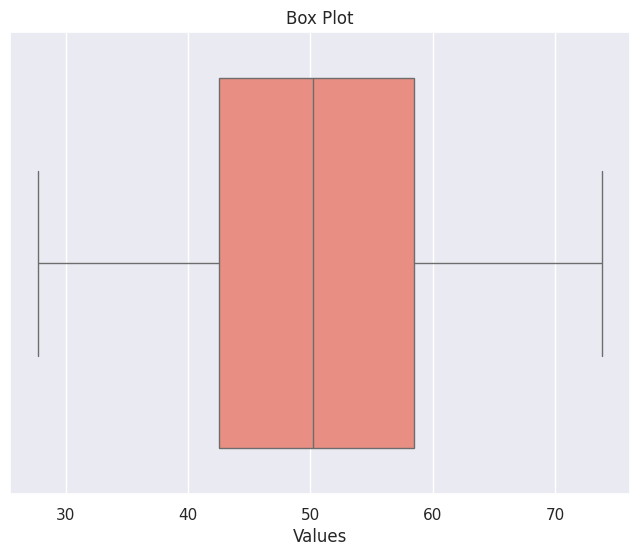
# Box Plot (Descriptive Statistics)
plt.figure(figsize=(8, 6))
sns.boxplot(data=data, orient='h', color='salmon')
plt.title('Box Plot')
plt.xlabel('Values')
plt.show()

Figure (3): Box Plot.

Inferential Statistics

Tests to perform on Data

Numerous statistical tests exist, each with specific assumptions and applications. We choose the right test based on data type, research question, and desired outcome. Some common tests are:

• One-Sample t-test: Tests whether the mean of a sample differs significantly from a known value.

• Two-Sample t-test: Tests whether the means of two samples differ significantly from each other.

• Chi-square test: Tests independence between categorical variables.

• ANOVA (Analysis of Variance): Tests whether the means of multiple groups are equal.

• Correlation analysis: Assess the strength and direction of the relationship between two variables.

# Inferential Statistics
## Perform a one-sample t-test to determine if the mean of the data is significantly different from a given value (e.g., 50)
t_statistic, p_value = stats.ttest_1samp(data, 50)
print("\nInferential Statistics:")
print("One-Sample t-test:")
print("T-statistic:", t_statistic)
print("P-value:", p_value)

# Output:
"""
Inferential Statistics:
One-Sample t-test:
T-statistic: 0.7886776690076842
P-value: 0.43218499762353
"""

# Confidence Interval (Inferential Statistics)
confidence_interval = stats.t.interval(0.95, len(data) - 1, 
                                    loc=np.mean(data), 
                                    scale=stats.sem(data))
print("95% Confidence Interval:", confidence_interval)

# Output:
"""
95% Confidence Interval: (48.75678325814636, 52.883476156810396)
"""

Let’s break down the parameters:

• 0.95: This is the confidence level for the interval. A 0.95 confidence level suggests that if we were to take 100 different samples and compute a 95% confidence interval for each sample, then approximately 95 of the 100 confidence intervals will contain the true mean value.

• len(data) - 1: This is the degrees of freedom, which is typically the sample size (in this case, the length of the data) minus 1.

• loc=np.mean(data): This is the location parameter, which is the mean of the data. The np.mean(data) function is used to calculate the mean of the data.

• scale=stats.sem(data): This is the scale parameter, which is the standard error of the mean of the data. The stats.sem(data) function is used to calculate the standard error of the mean.

Distribution

Data isn’t always scattered randomly; it doesn’t always follow a perfect bell curve (normal distribution). It often follows distinct patterns called distributions. Distributions describe the shape and spread of data. Understanding distributions helps choose appropriate analysis methods and interpret results accurately. Common distributions include:

• Normal distribution: Bell-shaped, with data clustered around the mean.

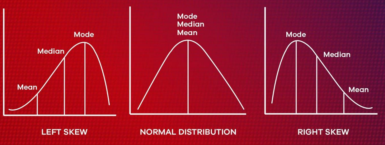
• Skewed distribution: Leans more towards one side, indicating more data points in a particular range.

• Uniform distribution: Data points spread evenly across a range.

• Bimodal distribution: Has two peaks, indicating two distinct groups of values.

Figure (4): Distribution Type.

Figure (5): Distribution Regarding M,M,M.

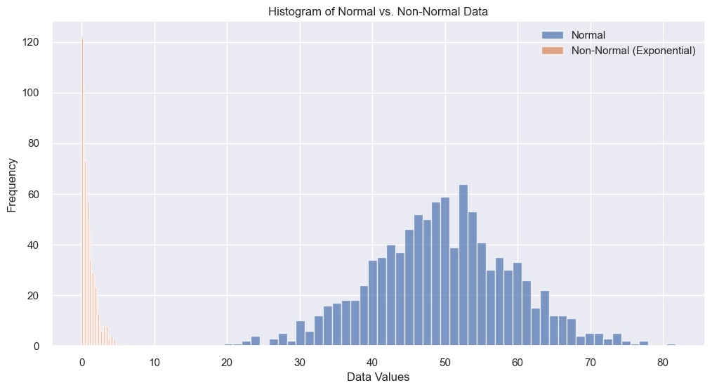
Normal Distribution vs. Non-Normal Distribution

Normal distribution (bell curve): Data points cluster around the mean, with fewer outliers. Think heights of adults.

Non-normal distributions: Data may be skewed to one side, have multiple peaks, or exhibit other unique shapes. Think about income levels or exam scores.

Different distributions impact analysis. Many statistical tests (like t-tests) assume a normal distribution. Analyzing non-normal data with these tests can lead to inaccurate conclusions. So, we should visually assess data normality with histograms or normal probability plots.

Alternatives for non-normal data:

• Transform the data: Make it closer to normal using mathematical functions.

• Use non-parametric tests: Designed for data without specific distributional assumptions (e.g., Wilcoxon signed-rank test, Kruskal-Wallis test).

# Generating data for normal and non-normal distributions
normal_data = np.random.normal(loc=50, scale=10, size=1000)
non_normal_data = np.random.exponential(scale=1, size=1000)

# Visualize distributions
plt.figure(figsize=(12, 6))
plt.hist(normal_data, label="Normal", bins=50, alpha=0.7)
plt.hist(non_normal_data, label="Non-Normal (Exponential)", bins=50, alpha=0.7)
plt.xlabel("Data Values")
plt.ylabel("Frequency")
plt.title("Histogram of Normal vs. Non-Normal Data")
plt.legend()
plt.grid(True)
plt.show()

# Normality tests
normality_test_normal = stats.shapiro(normal_data)
normality_test_non_normal = stats.shapiro(non_normal_data)

# Print normality test results
print("Normality test for normal data:")
print("Statistic:", normality_test_normal.statistic)
print("p-value:", normality_test_normal.pvalue)

print("\nNormality test for non-normal data:")
print("Statistic:", normality_test_non_normal.statistic)
print("p-value:", normality_test_non_normal.pvalue)

# Output:
"""
Normality test for normal data:
Statistic: 0.9990084767341614
p-value: 0.8774840831756592

Normality test for non-normal data:
Statistic: 0.8329999446868896
p-value: 4.50760282961232e-31
"""

Figure (6): Normal vs. Non-normal Distribution.

# Calculate statistics
normal_mean = np.mean(normal_data)
normal_mode = np.argmax(np.histogram(normal_data)[0])
normal_variance = np.var(normal_data)
normal_median = np.median(normal_data)
normal_q1 = np.quantile(normal_data, 0.25)
normal_q3 = np.quantile(normal_data, 0.75)

non_normal_mean = np.mean(non_normal_data)
non_normal_mode = np.argmax(np.histogram(non_normal_data)[0])
non_normal_variance = np.var(non_normal_data)
non_normal_median = np.median(non_normal_data)
non_normal_q1 = np.quantile(non_normal_data, 0.25)
non_normal_q3 = np.quantile(non_normal_data, 0.75)

# Identify outliers using IQR
def iqr_outliers(data):
    q1 = np.quantile(data, 0.25)
    q3 = np.quantile(data, 0.75)
    iqr = q3 - q1
    lower_bound = q1 - 1.5 * iqr
    upper_bound = q3 + 1.5 * iqr
    # return the outliers
    return data[~((data >= lower_bound) & (data <= upper_bound))]

# Using the iqr_outliers function
normal_outliers = iqr_outliers(normal_data)
non_normal_outliers = iqr_outliers(non_normal_data)

# Plot identified outliers
plt.figure(figsize=(12, 6))
plt.hist(normal_data, label="Normal", bins=50, alpha=0.7)
plt.hist(non_normal_data, label="Non-Normal (Exponential)", bins=50, alpha=0.7)

""" 
np.zeros_like(normal_outliers): This is the y-coordinates of the points in the scatter plot.
The np.zeros_like() function creates a new array of zeros with the same shape and type as the provided array (normal_outliers in this case).
So, all the points will be plotted on the x-axis (where y=0).
"""
plt.scatter(normal_outliers, np.zeros_like(normal_outliers),
        color='red', label='Normal Outliers')
plt.scatter(non_normal_outliers, np.zeros_like(non_normal_outliers),
        color='orange',label='Non-Normal Outliers')
plt.xlabel("Data Values")
plt.ylabel("Frequency")
plt.title("Distribution with Identified Outliers")
plt.legend()
plt.grid(True)
plt.show()

Figure (7): Normal vs. Non-normal Distribution With Outliers.

Sampling

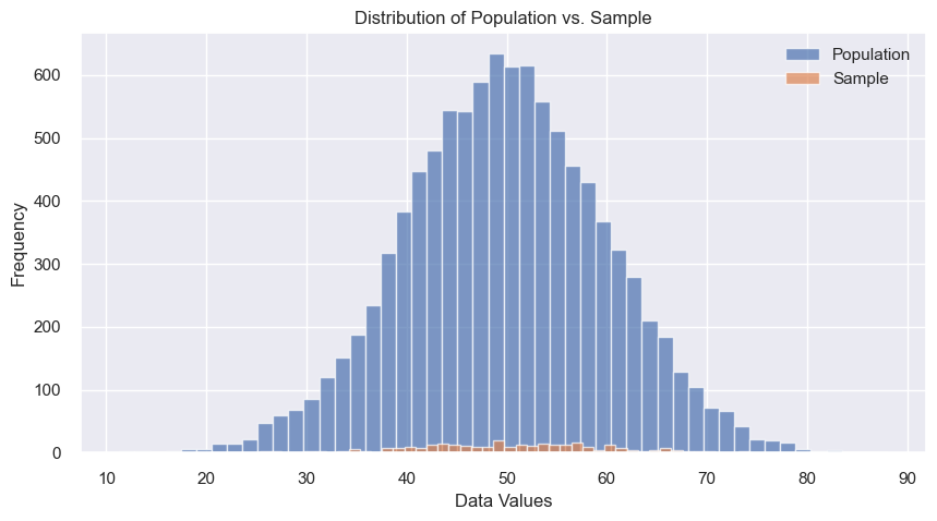
Analyzing entire populations is often impractical or impossible. We rely on representative samples (subsets) to draw inferences about the whole population. Different sampling methods exist:

• Simple random sampling: Each element has an equal chance of being chosen.

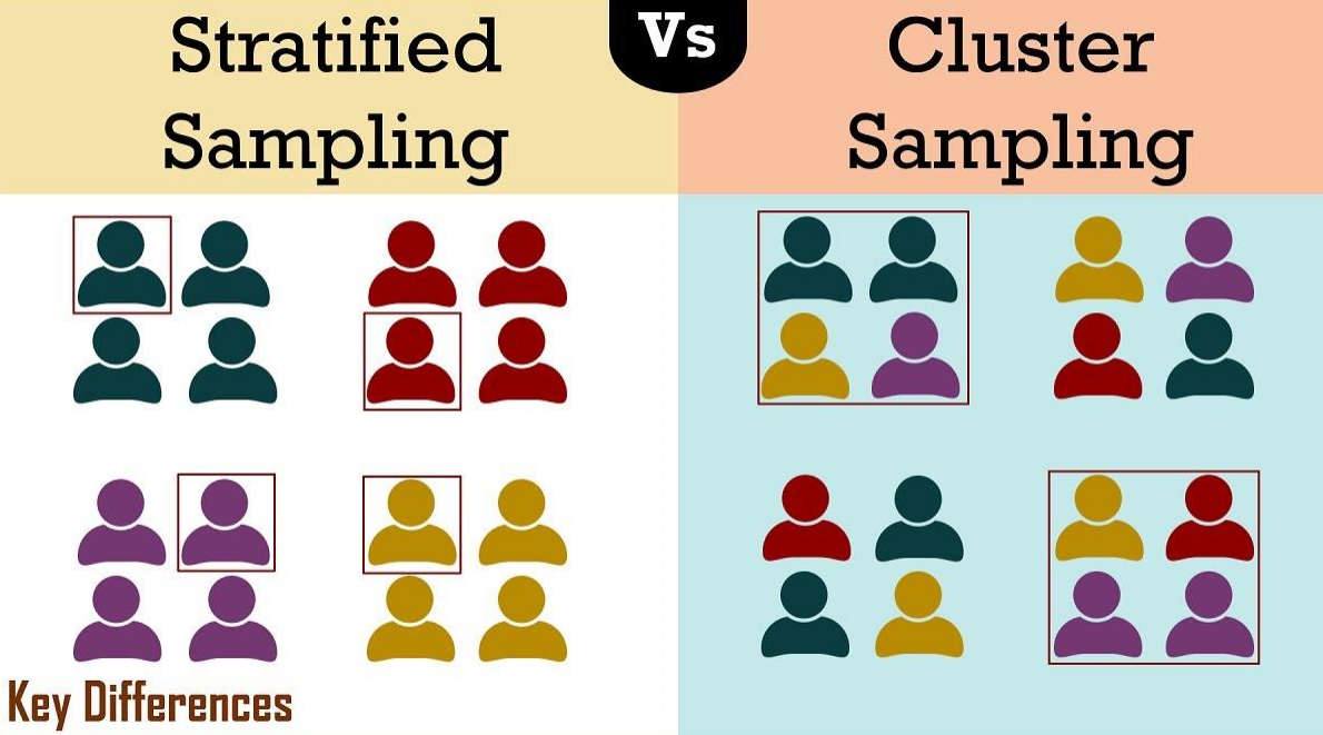
• Stratified sampling: Divides the population into subgroups (Strata) and selects samples from each stratum proportionally.

• Cluster sampling: Population divided into clusters, and entire clusters are randomly selected.

The sampling method significantly impacts the accuracy of conclusions drawn from the data.

Choosing the right method depends on the population characteristics and research question.

Figure (8): Stratified Sampling vs. Cluster Sampling.

# Generating a random sample from a population
population = np.random.normal(loc=50, scale=10, size=1000)
sample = np.random.choice(population, size=100, replace=False)
print("Sample Mean:", np.mean(sample))
print("population Mean:", np.mean(population))

# Output:
"""
Sample Mean: 51.37920400459694
population Mean: 50.215584286969616
"""

# Generate population and sample
population = np.random.normal(loc=50, scale=10, size=10000)
sample = np.random.choice(population, size=300, replace=False)

# Visualize sampling distribution
plt.figure(figsize=(10, 5))
plt.hist(population, label="Population", bins=50, alpha=0.7)
plt.hist(sample, label="Sample", bins=50, alpha=0.7)
plt.xlabel("Data Values")
plt.ylabel("Frequency")
plt.title("Distribution of Population vs. Sample")
plt.legend()
plt.grid(True)
plt.show()

Figure (9): Distribution of Population vs. Sample.

Performing Tests On Sample

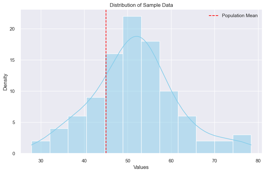
# using a one-sample t-test
data = np.random.normal(loc=50, scale=10, size=100)
population_mean = 45

t_statistic, p_value = stats.ttest_1samp(data, popmean=population_mean)
print("T-statistic:", t_statistic)
print("P-value:", p_value)

# Visualize the distribution of the sample data
plt.figure(figsize=(10, 6))
sns.histplot(data, kde=True, color='skyblue')
plt.axvline(x=population_mean, color='red', linestyle='--',
         label='Population Mean')
plt.title('Distribution of Sample Data')
plt.xlabel('Values')
plt.ylabel('Density')
plt.legend()
plt.show()

# Output:
"""
T-statistic: 6.727932727624613
P-value: 1.125213168893874e-09
"""

Figure (10): Distribution of Sample Data.

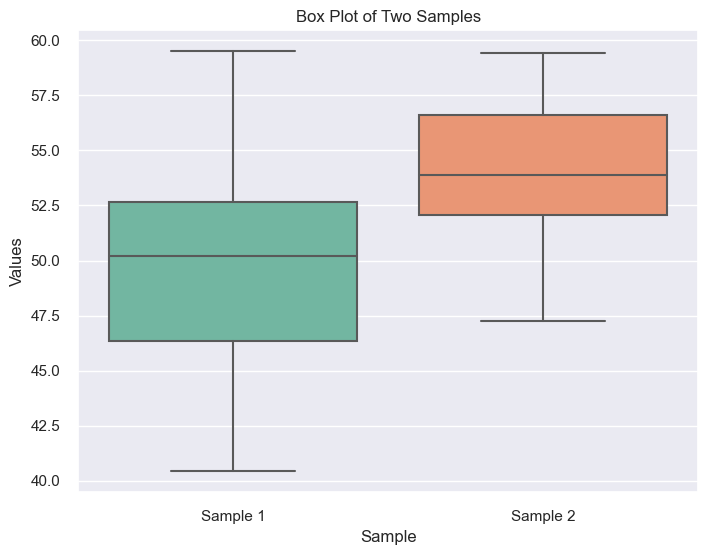
# using a two-sample t-test (compare means of two samples)
sample1 = np.random.normal(loc=50, scale=5, size=50)
sample2 = np.random.normal(loc=55, scale=3, size=50)

t_test_result = stats.ttest_ind(sample1, sample2)

print("\nT-test result (comparing means of two samples):", t_test_result)

# Visualize the distributions of the two samples using box plots
plt.figure(figsize=(8, 6))
sns.boxplot(data=[sample1, sample2], palette='Set2')
plt.title('Box Plot of Two Samples')
plt.xlabel('Sample')
plt.ylabel('Values')
plt.xticks(ticks=[0, 1], labels=['Sample 1', 'Sample 2'])

# Output:
"""
T-test result (comparing means of two samples):
Ttest_indResult(statistic=-5.515178839115084, pvalue=2.8345361343064335e-07)

"""
plt.show()

Figure (11): Box Plot of Two Samples.

Conclusion

This output provides information about a t-test comparing the means of two samples, Here’s a breakdown:

T-statistic: = -5.515

p-value: = 2.835e-07

Degrees of freedom: = 98

Explanation:

T-statistic: This value indicates the difference between the two sample means relative to the pooled standard deviation of the samples. A negative value suggests the first sample has a lower mean.

p-value: This is the probability of observing a difference as extreme or more extreme than the one found, assuming the null hypothesis H_0 (no difference in means) is true. A very small p-value (typically less than 0.05) suggests strong evidence against the null hypothesis, so we go with the alternative hypothesis H_1 (there is a difference in means).

Degrees of freedom: This reflects the number of independent observations contributing to the analysis (typically related to sample sizes).

In this case:

The negative t-statistic (-5.515): indicates the first sample has a lower mean compared to the second one.

The extremely small p-value (2.835e-07): strongly rejects the null hypothesis of no difference.

Based on this t-test result, we can confidently conclude that the means of the two samples are statistically different, with the first sample likely having a lower mean.

Notes:

it’s important to consider:

Direction of difference: The t-test only tells you there’s a difference, not which group has the higher mean.

Effect size: The t-statistic doesn’t quantify the magnitude of the difference. Consider additional analyses or visualizations for deeper insights.

Assumptions: Ensure the t-test assumptions (e.g., normality of errors, homogeneity of variances) are met for valid interpretation.