Power Prediction

17 minute read

Power Forecasting

Power prediction is important not only for the smooth and economic operation of a combined cycle power plant (CCPP) but also to avoid technical issues such as power outages.

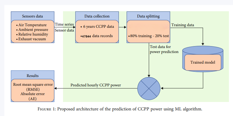
In this work, we propose to utilize machine learning algorithms to predict the hourly-based electrical power generated by a CCPP. For this, the generated power is considered a function of four fundamental parameters which are relative humidity, atmospheric pressure, ambient temperature, and exhaust vacuum.

The measurements of these parameters and their yielded output power are used to train and test the machine learning models. The dataset for the proposed research is gathered over a period of six years and taken from a standard and publicly available machine learning repository.

We predicting the net hourly electrical energy output (PE) of the plant using dataset from UCI Machine Learning Repository.

The accurate prediction of power generated by a plant helps in reducing various related issues such as power outages economic, and technical difficulties. In particular, an inaccurate prediction results in the rise of per unit cost of electric power due to the high fuel consumption. Hence, in this work, we aim at achieving a precise prediction of electric power of a base load CCPP on full load conditions thus ensuring decreased cost of per unit of electric power.

Proposed architecture

Figure (1): Proposed Architecture.

Technical Summary

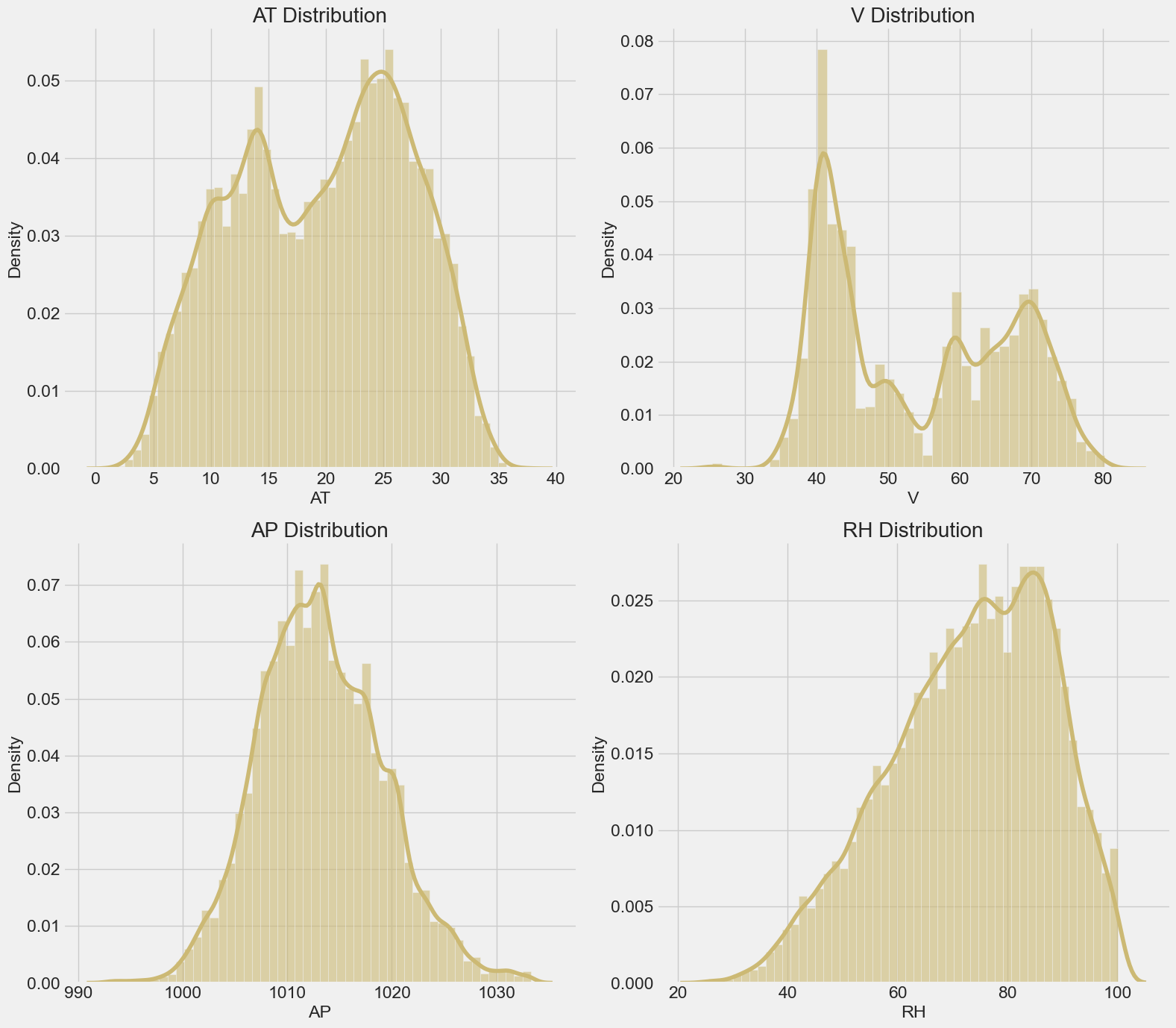
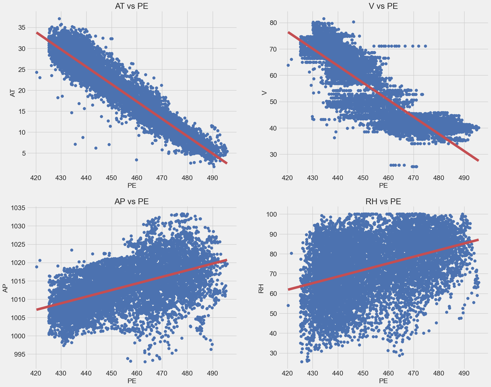
Data Exploration and Analysis: Ambient Pressure (AP) is nearly normaly distributed where Ambient Temperature (AT) and Vacuum (V) have multible peaks but Relative Humidity (RH) is left skewed. Target (PE) is highly positively correlated with RH and AP but is negatively correlated with AT and V.
Data Cleaning and Preprocessing: The dataset is cleaned by removing outliers and missing values. Data only contains 4 missing values for each parameter.Use IQR Method to remove outliers which was 500 instances. Use StandardScaler to normalize data. Split data into train, validaton and test sets.
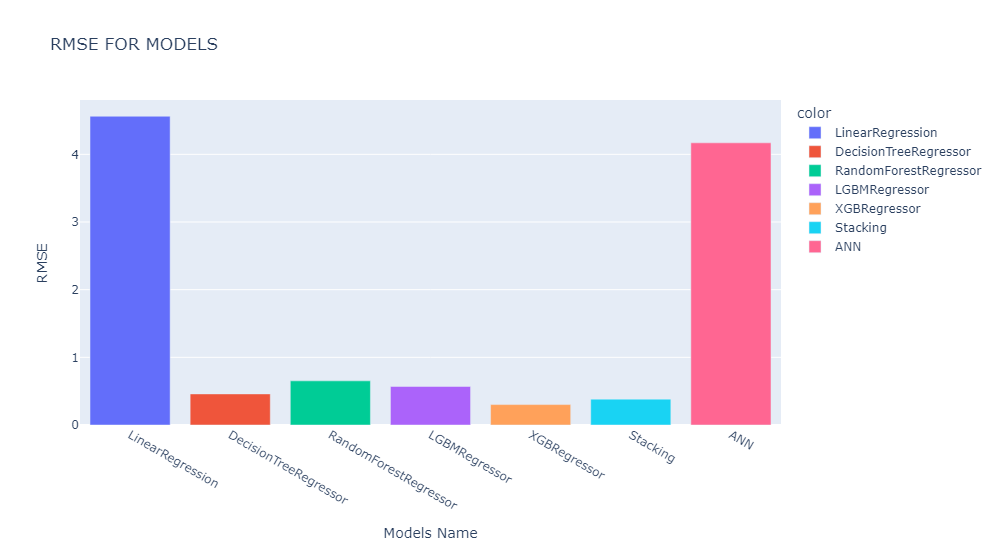
Machine Learning Models: Use Models like Linear Regression, Random Forest, Decision Tree, LightGBM, XGBoost,and Ensemble Voting. Use GridSearchCV to tune the hyperparameters of the models. The best model is XGBoost with RMSE of 0.30.
Artificial Neural Networks: Use deep neural networks with different architectures with a relu hidden layers. Use L2 regularization with Adam optimizer. More complex model, more bad result cuz of simpility and lack of the data.The best model is 1 hidden layers with 65 neurons with RMSE of 4.17.
Final Model: Use XGBoost with hyperparameters of learning_rate = 0.1, max_depth = 70, n_estimators = 500. The final model has RMSE of 0.30.
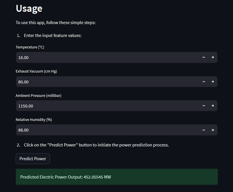
Deployment: Create a web application for the model using Streamlit. The web application is available at Check it out !.

Technical Analysis

Data Exploration and Analysis

Dataset

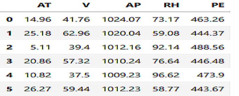
The dataset contains 47844 data points collected from a Combined Cycle Power Plant over 6 years (2006-2011) with 5 feature, when the power plant was set to work with full load. Features consist of hourly average ambient variables Ambient Temperature (AT), Ambient Pressure (AP), Relative Humidity (RH) and Exhaust Vacuum (V) to predict the net hourly electrical energy output (PE) of the plant.

Features consist of hourly average ambient variables :

Ambient Temperature (AT) in the range 1.81°C - 37.11°C
Ambient Pressure (AP) in the range 992.89 - 1033.30 milibar
Relative Humidity (RH) in the range 25.56% - 100.16%
Exhaust Vacuum (V) in the range 25.36 - 81.56 cm Hg
Net hourly electrical energy output (PE) 420.26 - 495.76 MW

Figure (2): Data.

Analysis

To estimate the mean, you will use:

\[\mu_i = \frac{1}{m} \sum_{j=1}^m x_i^{(j)}\]

to the variance you will use: $\sigma_i^2 = \frac{1}{m} \sum_{j=1}^m (x_i^{(j)} - \mu_i)^2$

Figure (3): Data Description.

As we see that the spread of thr AP is the smallest one which is due to the fact that the AP is nearly normaly distributed with the range of 992.89 - 1033.30 milibar.

let’s see the density plot of the data atrribute.

import warnings
# Filter and suppress warnings
warnings.filterwarnings("ignore")
# distribution of the variables
plt.style.use('fivethirtyeight')
fig, axes = plt.subplots(2, 2, figsize=(16, 14))

for axes, col in zip(axes.flatten(), df[:-1]):
      sns.distplot(df[col], ax=axes, kde=True,
      hist_kws={"alpha": 0.6},color='y').set(title=f"{col} Distribution")

plt.tight_layout()
sns.set(font_scale=1.5)
sns.despine()
plt.show()

Figure (4): Density Plot.

As we see that RH is left skewed where median is larger than the mean.

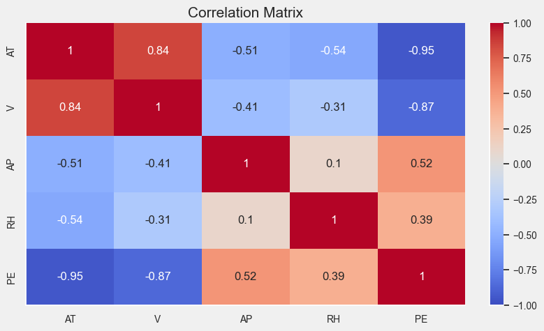
Let’s have a look at the correlation matrix to see if there is any correlation between the variables.

The variance: $var = \sigma_i^2 = \frac{1}{m} \sum_{j=1}^m (x_i^{(j)} - \mu_i)^2$

The Correlation Matrix: $cor(x,y) = (\frac{cov(x,y)}{\sqrt(var(x)var(y)})$

# correlation matrix
plt.style.use('fivethirtyeight')

sns.heatmap(df.corr(), annot=True, cmap='coolwarm',
             vmin=-1, vmax=1,annot_kws={"size": 12},
              cbar_kws={"fraction": 0.046})

plt.title("Correlation Matrix", fontsize=15)
sns.despine()
plt.show()

Figure (5): Correlation Matrix.

We can see from correlation matrix above that the v and AT features are highly correlated to the target variable but in negative correlation with PE.
We can see also that there is a strong positive correlation between V and AT

Some algorithms assume that there is a linear relationship between the variables as linear regression but some are not as decision trees and ensembles.

plt.style.use('fivethirtyeight')

for i, col in enumerate(df.columns[:-1]):
    plt.subplot(2, 2, i+1)
    sns.regplot(x="PE", y=col, data=df, scatter_kws={"color": "b"},
                line_kws={"color": "r"}).set(title=f"{col} vs PE")
    
sns.despine()
plt.show()

Figure (6): Linerar Relationship.

Data Cleaning and Preprocessing

Removing NAs

The dataset only have 4 missing values for each parameter. We will remove these rows as they are very few and removing them will not affect on the result.

df.isnull().sum()
AT    4
V     4
AP    4
RH    4
PE    4
dtype: int64

df.dropna(inplace=True)

Removing Outliers

Removing outliers is very important step to avoid the influence of the significant data point on the model. We will use IQR Method to remove outliers. The dataset is cleaned by removing outliers which was 500 instances.

let’s see the box plot of the data atrribute.

plt.style.use('fivethirtyeight')

for i, col in enumerate(df1.columns):
    plt.subplot(2, 3, i+1)
    sns.boxplot(df1[col],color='y',width=0.2,
                dodge=True,linewidth=2.5).set_title(col)

plt.tight_layout()
sns.set(font_scale=1.1)
sns.despine()
plt.show()

Figure (7): Box Plot for Outliers.

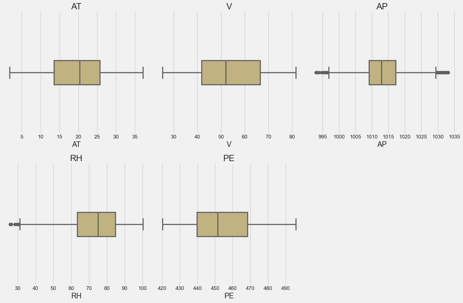
As we see that only AP and RH variable has outliers.

# Let's use the Percentiles or IQR Method 
q1 = df1.quantile(0.25)
q3 = df1.quantile(0.75)
iqr = q3 - q1

lower_bound = q1 - 1.5 * iqr
upper_bound = q3 + 1.5 * iqr

# save it in new dataframe
df2 = df1[((df1 > lower_bound) & (df1 < upper_bound)).all(axis=1)]

Normalizing Data

We use the StandardScaler from sklearn.preprocessing to normalize the data.

The z-score is given by the equation:

\[z = \frac{x - \mu}{\sigma}\]

The normalization is very important method for model convergence.

Data Splitting

We use the train_test_split from sklearn.model_selection to split the data into training, validation and testing sets.

The splititng is 60% training, 20% validation and 20% testing.

Splitting the data into training, validation and testing sets is very important for model evaluation. where we use validation set to evaluate the model performance to avoid overfitting and make model selection with hyperparameter tuning and optimization.

We can use cross validation to evaluate the model performance and select the best model if you have not enough data to use validation set and use only train and test set but i didn’t use it here.

Machine Learning Models

The equation for the cost function with multiple variables $J(\mathbf{w},b)$ is:

$J(\mathbf{w},b) = \frac{1}{2m} \sum\limits_{i = 0}^{m-1} (f_{\mathbf{w},b}(\mathbf{x}^{(i)}) - y^{(i)})^2 \tag{1}$ where: $f_{\mathbf{w},b}(\mathbf{x}^{(i)}) = \mathbf{w} \cdot \mathbf{x}^{(i)} + b \tag{2}$

Gradient descent for multiple variables:

\[\begin{align*} \text{repeat}&\text{ until convergence:} \; \lbrace \newline\; & w_j = w_j - \alpha \frac{\partial J(\mathbf{w},b)}{\partial w_j} \tag{3} \; & \text{for j = 0..n-1}\newline &b\ \ = b - \alpha \frac{\partial J(\mathbf{w},b)}{\partial b} \newline \rbrace \end{align*}\]

where, n is the number of features, parameters $w_j$, $b$, are updated simultaneously and where

\[\begin{align} \frac{\partial J(\mathbf{w},b)}{\partial w_j} &= \frac{1}{m} \sum\limits_{i = 0}^{m-1} (f_{\mathbf{w},b}(\mathbf{x}^{(i)}) - y^{(i)})x_{j}^{(i)} \tag{4} \\ \frac{\partial J(\mathbf{w},b)}{\partial b} &= \frac{1}{m} \sum\limits_{i = 0}^{m-1} (f_{\mathbf{w},b}(\mathbf{x}^{(i)}) - y^{(i)}) \tag{5} \end{align}\]

Define the Root Mean Squared Error (RMSE):

def RMSE(y,y_hat):
  return np.sqrt(mean_squared_error(y,y_hat))

Linear Regression

Let’s use the simplest base model and see what we can get out of it. it’s important to start with simple models in the beginning and then move to more complex models to see if you can get better results or not.

from sklearn.linear_model import LinearRegression
linear_model = LinearRegression()
# fit on train data
model_fit = linear_model.fit(X_train_scaled,y_train)

# predict on train data
prediction = model_fit.predict(X_val_scaled)

RMSE(y_val,prediction)

RMSE: 4.56 

Random Forest

let’s try some random forest hyperparameters tuning to see if we can get better results.

min_samples_split_list = [2,10, 30, 50, 100, 200, 400, 700, 1000]
max_depth_list = [1,2, 3, 4, 7, 8, 16, 32, 64, None] # None means that there is no depth limit.
n_estimators_list = [10,50,100,500]


RMSE_list_train = []
RMSE_list_val = []

for min_samples_split in min_samples_split_list:

    # fit the model
    model = RandomForestRegressor(min_samples_split = min_samples_split,random_state = 42).fit(X_train_scaled,y_train)

    predictions_train = model.predict(X_train_scaled) ## The predicted values for the train dataset
    predictions_val = model.predict(X_val_scaled) ## The predicted values for the test dataset
    RMSE_train = RMSE(y_train,predictions_train)
    RMSE_val = RMSE(y_val,predictions_val)
    RMSE_list_train.append(RMSE_train)
    RMSE_list_val.append(RMSE_val)

plt.title('Train vs Validation metrics')
plt.xlabel('min_samples_split')
plt.ylabel('RMSE')
plt.xticks(ticks = range(len(min_samples_split_list )),labels=min_samples_split_list)
plt.plot(RMSE_list_train)
plt.plot(RMSE_list_val)
plt.legend(['Train','Validation'])

Figure (8): Random Forest with min_samples_split.

RMSE_list_train = []
RMSE_list_val = []

for max_depth in max_depth_list:

    # fit the model
    model = RandomForestRegressor(max_depth = max_depth,random_state = 42).fit(X_train_scaled,y_train)

    predictions_train = model.predict(X_train_scaled) ## The predicted values for the train dataset
    predictions_val = model.predict(X_val_scaled) ## The predicted values for the validation dataset
    RMSE_train = RMSE(y_train,predictions_train)
    RMSE_val = RMSE(y_val,predictions_val)
    RMSE_list_train.append(RMSE_train)
    RMSE_list_val.append(RMSE_val)

plt.title('Train vs Validation metrics')
plt.xlabel('max_depth')
plt.ylabel('RMSE')
plt.xticks(ticks = range(len(max_depth_list )),labels=max_depth_list)
plt.plot(RMSE_list_train)
plt.plot(RMSE_list_val)
plt.legend(['Train','Validation'])

Figure (9): Random Forest with max_depth.

RMSE_list_train = []
RMSE_list_val = []

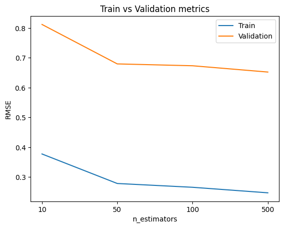
for n_estimators in n_estimators_list:

    # fit the model
    model = RandomForestRegressor(n_estimators = n_estimators,random_state = 42).fit(X_train_scaled,y_train)

    predictions_train = model.predict(X_train_scaled) ## The predicted values for the train dataset
    predictions_val = model.predict(X_val_scaled) ## The predicted values for the validation dataset
    RMSE_train = RMSE(y_train,predictions_train)
    RMSE_val = RMSE(y_val,predictions_val)
    RMSE_list_train.append(RMSE_train)
    RMSE_list_val.append(RMSE_val)

plt.title('Train vs Validation metrics')
plt.xlabel('n_estimators')
plt.ylabel('RMSE')
plt.xticks(ticks = range(len(n_estimators_list )),labels=n_estimators_list)
plt.plot(RMSE_list_train)
plt.plot(RMSE_list_val)
plt.legend(['Train','Validation'])

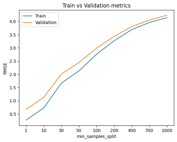
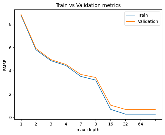
Figure (10): Random Forest with n_estimators.

As we see from above figures that the best parameters are min_samples_split = 2, max_depth = 64, n_estimators = 500.

# Create the RandomForestRegressor
RandomForest_model = RandomForestRegressor(n_estimators=500,
                                           min_samples_split = 2,
                                             max_depth = 64,
                                             random_state = 42).fit(X_train_scaled,y_train)

RMSE(y_val, RandomForest_model.predict(X_val_scaled))

RMSE: 0.6522

Decision Tree

from sklearn.tree import DecisionTreeRegressor
# Create the Decision Tree Regressor
decision_tree_model = DecisionTreeRegressor(min_samples_split = 2,
                                             max_depth = 64,
                                             random_state = 42).fit(X_train_scaled,y_train)

RMSE(y_val, decision_tree_model.predict(X_val_scaled))

RMSE: 0.4593

let’s use GridSearchCV to tune the hyperparameters of the following models.

LightGBM

# use GridSearchCV to get best hyperparameter
lgb_params = {
    'n_estimators':[10,50,200,500,700],
    'max_depth':[5,20,40,65,70],
    'learning_rate':[0.01,0.1,0.9,1],
    'random_state':[42],
    'class_weight':['balanced'],
}

# Create the RMSE scorer
rmse_scorer = make_scorer(lambda y_true, y_pred: np.sqrt(mean_squared_error(y_true, y_pred)),
                           greater_is_better=False)

lgb_rg = GridSearchCV(LGBMRegressor(),
                      lgb_params,
                      scoring = rmse_scorer,
                      verbose=0
                     )

lgb_rg.fit(X_train_scaled,y_train)

print(lgb_rg.best_params_)

Best parameters:

{'class_weight': 'balanced', 'learning_rate': 0.9, 'max_depth': 20, 'n_estimators': 700}

lgb_clf = LGBMRegressor(class_weight = 'balanced',
                             learning_rate = 0.9,
                             max_depth = 20,
                             n_estimators = 700,
                             random_state = 42,
                             )
lgb_clf.fit(X_train_scaled, y_train,
            eval_set = [(X_train_scaled, y_train),(X_val_scaled, y_val)],
            early_stopping_rounds = 300,
            verbose=1,
            eval_metric='rmse'
           )

RMSE: 0.5692

XGBoost

# use GridSearchCV to get best hyperparameter
xgb_params = {
    'n_estimators':[10,50,200,500,700],
    'max_depth':[5,20,40,65,70],
    'learning_rate':[0.01,0.1,0.9,1],
    'random_state':[42],
}

# Create the RMSE scorer
rmse_scorer = make_scorer(lambda y_true, y_pred: np.sqrt(mean_squared_error(y_true, y_pred)),
                           greater_is_better=False)

xgb_rg = GridSearchCV(XGBRegressor(),
                      xgb_params,
                      scoring = rmse_scorer,
                      verbose=0
                     )

xgb_rg.fit(X_train_scaled,y_train)

print(xgb_rg.best_params_)

Best parameters:

  {'learning_rate': 0.1, 'max_depth': 70, 'n_estimators': 500}

xgb_rg = XGBRegressor(learning_rate = 0.1,
                             max_depth = 70,
                             n_estimators = 500,
                             random_state = 42,
                             )
xgb_rg.fit(X_train_scaled, y_train,
            eval_set = [(X_val_scaled, y_val)],
            early_stopping_rounds = 300,
            verbose=1,
            eval_metric=['rmse','mae']
           )
RMSE: 0.3018

Ensemble Voting

from sklearn.ensemble import VotingRegressor


voting_rg = VotingRegressor(estimators = [
    ('Dt',decision_tree_model ),
    ('rf',RandomForest_model ),
    ('lgb',lgb_clf),
    ('xgb',xgb_rg),
    ])

voting_rg.fit(X_train_scaled, y_train)

RMSE(y_val, voting_rg.predict(X_val_scaled))

RMSE: 0.3815

We not get better results than the XGBoost models.

Artificial Neural Networks

We will try to use different architectures of deep neural networks with a relu as a hidden layers. the model with regularization, We will use L2 regularization. We use Adam optimizer as the optimizer.

The equation for the cost function with regularization is:

$J(\mathbf{w},b) = \frac{1}{2m} \sum\limits_{i = 0}^{m-1} (f_{\mathbf{w},b}(\mathbf{x}^{(i)}) - y^{(i)})^2 + \frac{\lambda}{2m} \sum_{j=0}^{n-1} w_j^2 \tag{1}$ where: $f_{\mathbf{w},b}(\mathbf{x}^{(i)}) = \mathbf{w} \cdot \mathbf{x}^{(i)} + b \tag{2}$

Gradient descent with regularization is:

$\begin{align*} &\text{repeat until convergence:} \; \lbrace \\ & \; \; \;w_j = w_j - \alpha \frac{\partial J(\mathbf{w},b)}{\partial w_j} \tag{3} \; & \text{for j := 0..n-1} \\ & \; \; \; \; \;b = b - \alpha \frac{\partial J(\mathbf{w},b)}{\partial b} \\ &\rbrace \end{align*}$ Where each iteration performs simultaneous updates on $w_j$ for all $j$.

The gradient calculation

\[\begin{align*} \frac{\partial J(\mathbf{w},b)}{\partial w_j} &= \frac{1}{m} \sum\limits_{i = 0}^{m-1} (f_{\mathbf{w},b}(\mathbf{x}^{(i)}) - y^{(i)})x_{j}^{(i)} + \frac{\lambda}{m} w_j \tag{4} \\ \frac{\partial J(\mathbf{w},b)}{\partial b} &= \frac{1}{m} \sum\limits_{i = 0}^{m-1} (f_{\mathbf{w},b}(\mathbf{x}^{(i)}) - y^{(i)}) \tag{5} \end{align*}\]

# set seed for reproducibility
tf.random.set_seed(1234)

# Define a list of layer architectures to try
layer_architectures = [

    [Dense(units = 40, activation='relu', name = 'L1', input_shape=(4,)),
     Dense(units = 1, name = 'L11')],

    [Dense(units = 65, activation='relu', name = 'L2222', input_shape=(4,)),
     Dense(units = 1, name = 'L22222')],

     [Dense(units = 65, activation='relu', name = 'L999999', input_shape=(4,)),
      Dense(units = 25, activation='relu', name = 'L99999'),
      Dense(units = 1, name = 'L9999')],

    [Dense(units = 65, activation='relu',
           kernel_regularizer = tf.keras.regularizers.l2(0.1),
           name = 'L2', input_shape=(4,)),
     Dense(units = 1, name = 'L22')],

     [Dense(units = 65, activation='relu',
            kernel_regularizer = tf.keras.regularizers.l2(0.1),
            name = 'L9', input_shape=(4,)),
      Dense(units = 25, activation='relu',
            kernel_regularizer = tf.keras.regularizers.l2(0.1), name = 'L99'),
      Dense(units = 1, name = 'L999')],

    [Dense(units = 125, activation='relu',
           kernel_regularizer = tf.keras.regularizers.l2(0.1),
           name = 'L3', input_shape=(4,)),
     Dense(units = 65, activation='relu',
           kernel_regularizer = tf.keras.regularizers.l2(0.1),
           name = 'L33'),
     Dense(units = 1, name = 'L333')],

    [Dense(units = 65, activation='relu',
           kernel_regularizer = tf.keras.regularizers.l2(0.1),
           name = 'L4', input_shape=(4,)),
     Dense(units = 64, activation='relu',
           kernel_regularizer = tf.keras.regularizers.l2(0.1),
           name = 'L44'),
     Dense(units = 1, name = 'L444')],


    [Dense(units = 125, activation='relu',
           kernel_regularizer = tf.keras.regularizers.l2(0.1),
           name = 'L5', input_shape=(4,)),
     Dense(units = 64, activation='relu',
           kernel_regularizer = tf.keras.regularizers.l2(0.1),
           name = 'L55'),
     Dense(units = 1, name = 'L555')],


    [Dense(units = 164, activation='relu',
           kernel_regularizer = tf.keras.regularizers.l2(0.1),
           name = 'L6', input_shape=(4,)),
     Dense(units = 125, activation='relu',
           kernel_regularizer = tf.keras.regularizers.l2(0.1),
           name = 'L66'),
     Dense(units = 64, activation='relu',
           kernel_regularizer = tf.keras.regularizers.l2(0.1),
           name = 'L666'),
     Dense(units = 1, name = 'L6666')],

    [Dense(units = 200, activation='relu',
           kernel_regularizer = tf.keras.regularizers.l2(0.1),
           name = 'L7', input_shape=(4,)),
     Dense(units = 164, activation='relu',
           kernel_regularizer = tf.keras.regularizers.l2(0.1),
           name = 'L77'),
     Dense(units = 125, activation='relu',
           kernel_regularizer = tf.keras.regularizers.l2(0.1),
           name = 'L777'),
     Dense(units = 64, activation='relu',
           kernel_regularizer = tf.keras.regularizers.l2(0.1),
           name = 'L7777'),
     Dense(units = 1, name = 'L77777')],

    [Dense(units = 300, activation='relu',
           kernel_regularizer = tf.keras.regularizers.l2(0.1),
           name = 'L8', input_shape=(4,)),
     Dense(units = 200, activation='relu',
           kernel_regularizer = tf.keras.regularizers.l2(0.1),
           name = 'L88'),
     Dense(units = 164, activation='relu',
           kernel_regularizer = tf.keras.regularizers.l2(0.1),
           name = 'L888'),
     Dense(units = 125, activation='relu',
           kernel_regularizer = tf.keras.regularizers.l2(0.1),
           name = 'L8888'),
     Dense(units = 64, activation='relu',
           kernel_regularizer = tf.keras.regularizers.l2(0.1),
           name = 'L88888'),
     Dense(units = 1, name = 'L888888')],

    # Add more layer configurations as desired
]

best_model = None
best_loss = float('inf')

# Loop over each layer architecture and train/evaluate the model
for architecture in layer_architectures:
    model = tf.keras.Sequential(architecture)

    # Compile the model
    model.compile(optimizer= Adam(learning_rate=0.01), loss= MeanSquaredError())
    # Fit the model
    model.fit(X_train_scaled, y_train, epochs=50, verbose=0)
    # Predict
    y_pred = model.predict(X_val_scaled)

    loss = RMSE(y_val, y_pred)

    print(f"Architecture: {architecture}")
    print(f"Loss: {loss:.4f}")

    # Track the best model based on the lowest loss
    if loss < best_loss:
        best_loss = loss
        best_model = model


        
print(f'<-- best_loss: {best_loss}')

best_loss: 4.17 

The best model was the second one with 1 hidden layer of 65 units without regularization.

Final Result

The best model is XGBoost with hyperparameters of learning_rate = 0.1, max_depth = 70, n_estimators = 500. The final model has RMSE of 0.30.

Figure (11): Final Result.

Deployment

Create a web application for the model using Streamlit.

# import the necessary libraries
import streamlit as st
import pandas as pd
import numpy as np
import pickle
import os
from sklearn.preprocessing import StandardScaler


# Load the trained machine learning model
@st.cache_data
def load_model():
    pickle_path = os.path.join(os.getcwd(), 'models','xgb_model.pkl')
    with open(pickle_path, 'rb') as f:
        the_model = pickle.load(f)
    return the_model
model = load_model()

# Load the trained scaling
@st.cache_data
def load_scaler():
    scaler_path = os.path.join(os.getcwd(), 'models','scaler.pkl')
    with open(scaler_path, 'rb') as f:
        scaler = pickle.load(f)
    return scaler
scaler = load_scaler()

# Define the Streamlit app layout
st.title('Combined Cycle Power Plant Power Prediction')
st.markdown('Welcome to the Combined Cycle Power Plant Power Prediction Web App! '
            'This app utilizes the XGBoost algorithm to predict the electric power output of a combined cycle power plant.')

st.markdown('## About Combined Cycle Power Plants')
st.markdown('Combined cycle power plants are a type of power generation facility that produce electricity through a combination of gas and steam turbines. '
            'They are known for their high efficiency and low emissions, making them an important component of the energy landscape.')

st.markdown('## Power Prediction with XGBRegressor')
st.markdown('XGBRegressor is a powerful machine learning algorithm widely used for regression tasks. '
            'It excels in capturing complex relationships between input features and target variables, making it suitable for predicting power output in this context.')

st.markdown('## Usage')
st.markdown('To use this app, follow these simple steps:')

st.markdown('1. Enter the input feature values:')
feature1 = st.number_input('Temperature (°C)', min_value=0.0)
feature2 = st.number_input('Exhaust Vacuum (cm Hg)', min_value=0.0)
feature3 = st.number_input('Ambient Pressure (millibar)', min_value=0.0)
feature4 = st.number_input('Relative Humidity (%)', min_value=0.0)

st.markdown('2. Click on the "Predict Power" button to initiate the power prediction process.')

# Create a button to trigger the prediction
if st.button('Predict Power'):
    
    input_features = np.array([[feature1, feature2, feature3, feature4]])
    
    # Scale the input features  
    scaled_features = scaler.transform(input_features)  
    
    # Make the prediction using the loaded model
    prediction = model.predict(scaled_features)

    # Display the predicted power value to the user
    st.success(f'Predicted Electric Power Output: {prediction[0]:.5f} MW')


st.markdown('## Get Started')
st.markdown('To get started, make sure you have the necessary input feature values ready. '
            'Then, simply input the values, and let the app perform the power prediction for you.')

Figure (12): Web Application.

Reference

Pınar Tüfekci, Çorlu Faculty of Engineering, Namık Kemal University, TR-59860 Çorlu, Tekirdağ, Turkey Email: ptufekci @ nku.edu.tr
Heysem Kaya, Department of Computer Engineering, Boğaziçi University, TR-34342, Beşiktaş, İstanbul, Turkey Email: heysem @ boun.edu.tr
https://www.hindawi.com/journals/wcmc/2021/9966395/
https://archive.ics.uci.edu/dataset/294/combined+cycle+power+plant

Abdelrahman El-Nabawy